
ECON 121 Discussion: Week 10
Slides available here:
All discussion slides here:

Reminders
Next week is 🌴 spring break 🌴
- There will be no lectures, discussion sections, office hours, etc.
Midterm #2 will be on April 4th in class
This is the Friday after spring break
Midterm #2 will cover all chapters and Dr. Pieper’s material since Midterm #1: it is not cumulative
- We have not covered all Midterm #2 material yet: Dr. Pieper will decide what material is covered closer to the exam date
Come to office hours with any questions and for help with studying!
My advice: start studying now - it’s much easier to study over a longer period of time than cramming in the week before the exam!
Today’s Plan
- Review consumption spending and “the multiplier” effect of consumption spending
- Practice problems
Consumption and the GDP Multiplier
Consumption Spending
Consumption is really, really, REALLY important for economic growth and the overall health of an economy
Over two thirds of spending on final goods and services in the U.S. is consumption spending
How much consumers spend largely depends on two things:
Current disposable income: how much money consumers have to spend after paying taxes and recieving government transfers
- Government transfers: social security checks, welfare benefits, etc.
Marginal propensity to consume (MPC): if you had an extra dollar, how much more would you consume?
\[ \text{MPC} = \frac{\Delta \text{ Consumer Spending}}{\Delta \text{ Disposable Income}} \]
- If you save the whole dollar, your MPC would be 0!
- If you spend the whole dollar, your MPC would be 1!
MPC And MPS
MPC tells us how much consumption spending will change if people have more disposable income:
\[ \text{MPC} = \frac{\Delta \text{ Consumer Spending}}{\Delta \text{ Disposable Income}} \implies \text{MPC} \times \Delta \text{ Disposable Income} = \Delta \text{ Consumer Spending} \]
Intuition: when disposable income goes up by $X, consumption spending goes up by $X \(\times\) MPC!
If you’re not spending… you’re saving! So if we know the MPC we also know the marginal propensity to save (MPS)
\[ MPS = 1 - MPC \]
MPC And The Consumption Function
A simple model for studying how much a household spends on consumption:
\[ \text{Consumer Spending} = \text{Base Spending} + \text{MPC} \times \text{Disposable Income} \]
The book uses \(c = a + MPC \times yd\)… same thing
Notice: we can graph the consumption function as a line
“Base Spending” = the intercept, how much the household would consume with $0 in income
MPC = the slope, how much consumer spending changes as disposable income changes
The point: how much consumption there is is very strongly related to how much disposable income people have and this is not a 1:1 relationship since it depends on how likely consumers are to spend that money on consumer goods and services
The GDP Multiplier: An Example
If consumption spending depends on the level of disposable income and MPC, how does this affect GDP? Does a change in \(G\), \(I\), \(IM\), or \(X\) in one year only affect GDP that year?
Say \(G\) (and so also GDP) increases by $1 billion in 2025 and consumers MPS is 0.2. Does this affect GDP in 2026? 2027? Etc.?
In 2026 people will spend 80% of that increase in GDP on consumption, increasing 2026 GDP:
\[ MPC \times \$1 \text{ billion} = 0.8 \times \$1 \text{ billion} = \$800 \text{ million} \]
Then in 2027 they’ll spend 80% of that on consumption (on top of whatever 2027 consumption would have been):
\[ MPC \times \$800 \text{ million} = 0.8 \times \$800 \text{ million} = \$640 \text{ million} \]
If you do this infinity times, you end up with a chain reaction that totals $5 billion higher GDP across time:
\[ \frac{1}{1 - MPC} \times \$1 \text{ billion} = \frac{1}{MPS} \times \$1 \text{ billion} = \frac{1}{0.2} \times \$1 \text{ billion} = \$5 \text{ billion} \]
Practice Problems
Practice Problem #1
Why does the GDP multiplier exist?
- When people spend money, that money ends up in the pockets or bank accounts of other people or organizations, who then use that money in some way.
- When people see the government spending more money, they realize that the government thinks that prices are low; thus, they believe it is a good time to buy things
- When people see other people spending money, they know that the economy is about to improve, leading them to spend more money.
- The multiplier exists because money spent today is always more valuable than money spent in the future, due to inflation and interest rates.
Answer
Your spending is someone else’s income. And then that person’s able to spend, which becomes someone else’s income. And so on and so on.
If your ability to spend changes because of an increase in GDP (aggregate spending), this makes up the multiplier effect we talked about earlier.
Practice Problem #2
Which would result in a larger change in output for some change in expenditure: a higher MPC or a lower MPC? Try to explain your answer both mathematically and economically.
Hint: remember the multiplier
\[ \frac{1}{MPS} \text{ or } \frac{1}{1 - MPC} \]
Practice Problem #2
Which would result in a larger change in output for some change in expenditure: a higher MPC or a lower MPC? Try to explain your answer both mathematically and economically.
Hint: remember the multiplier
\[ \frac{1}{MPS} \text{ or } \frac{1}{1 - MPC} \]
Answer
A higher MPC would lead to a larger change in output.
The math: for the multiplier to be large, we want the denominator to be small. This happens if MPC is large (so then MPS would be small).
The economics: if, in the last answer, your MPC was low and you spent less of your money and saved it instead then “your expenditure is someone else’s income” doesn’t really work since your expenditure is lower! A higher MPC makes the multiplier effect larger.
Practice Problem #3
Use the word bank to fill in the blanks.
The consumption function tells us the relationship between _____ and _____. The slope of the consumption function is _____.
If your MPC is 0.9 and your disposable income this year increases by $2,000, your consumption spending this year would increase by _____.
Word Bank
- $2,000
- how much you would spend if you make $0
- disposable income
- $1,800
- negative
- MPC
- inflation
- consumption spending
- $0
Practice Problem #3
Use the word bank to fill in the blanks.
The consumption function tells us the relationship between consumption spending and disposable income. The slope of the consumption function is MPC.
If your MPC is 0.9 and your disposable income this year increases by $2,000, your consumption spending this year would increase by $1,800.
Word Bank
- $2,000
- how much you would spend if you make $0
disposable income$1,800- negative
MPC- inflation
consumption spending- $0
Practice Problem #4
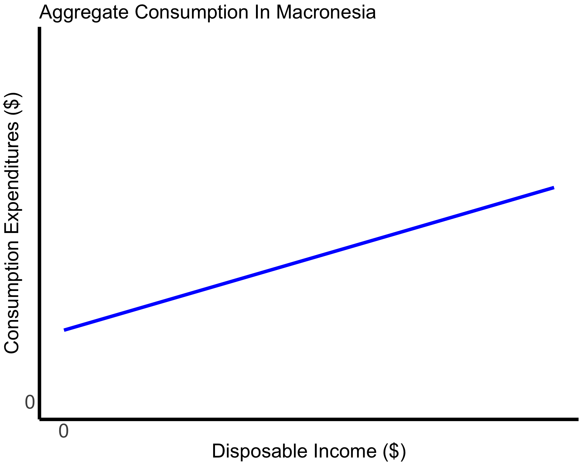
The aggregate consumption function for the country of Macronesia is plotted to the right.
Macronesia’s largest company, Acme Inc., just announced plans to build several new factories next year. Would this change Macronesians’ expectations about their disposable income? If so, how? Would this change aggregate consumption expenditures? If so, show how on the graph.
Practice Problem #4
The aggregate consumption function for the country of Macronesia is plotted to the right.
Macronesia’s largest company, Acme Inc., just announced plans to build several new factories next year. Would this change Macronesians’ expectations about their disposable income? If so, how? Would this change aggregate consumption expenditures? If so, show how on the graph.
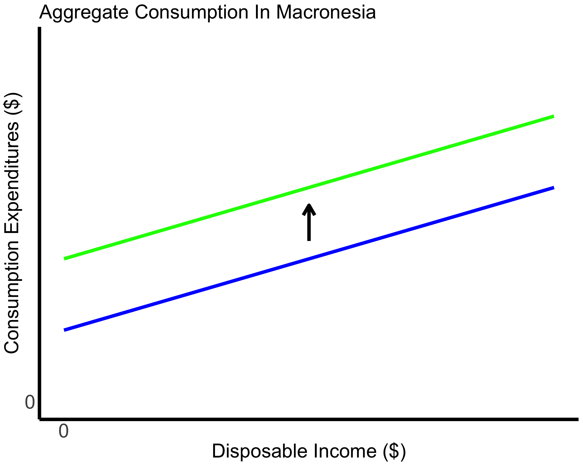
Answer
Investment spending will raise GDP and Macronesians’ expectations for future disposable income. This should increase aggregate consumption expenditures (which will shift the curve on the graph upward).
Practice Problem #5
Aggregate expenditures in Macronesia just increased by $10 billion. Macronesians’ marginal propensity to save is 0.3. Overall, what’s the change in Macronesia’s real GDP after the increase in aggregate expenditures?
Practice Problem #5
Aggregate expenditures in Macronesia just increased by $10 billion. Macronesians’ marginal propensity to save is 0.3. Overall, what’s the change in Macronesia’s real GDP after the increase in aggregate expenditures?
Answer
Remember: someone’s expenditure is another person’s income. So an increase in aggregate expenditures is an increase in disposable income.
\[ \frac{1}{MPS} \times \text{ Aggregate Expenditures} \]
\[ \frac{1}{.3} \times \$10 \text{ billion} = 3.\bar{3} \times \$10 \text{ billion} = \$33.\bar{3} \text{ billion} \]